This document outlines a method which can be used to display service contours and interference contours in the same map window in order to identify areas of overlap. For this example, we will use an existing TV transmitter (DTV) as the service transmitter and several land/mobile radio (LMR) transmitters as the interfering transmitters. We will also demonstrate how to identify the affected population (number of households) within the DTV/LMR contour overlap using a Demographic study.
TX information used to setup study
For DTV
Channel 10
TV Service Contour Field = 36 dBµV/m
TV service Contour % Time = 90
For LMR
Channel 10
Interferer Contour Field = 46 dBµV/m
Interferer Contour % Time = 10
Step-by-step guide
Set up and configuration for the DTV and LMR sites
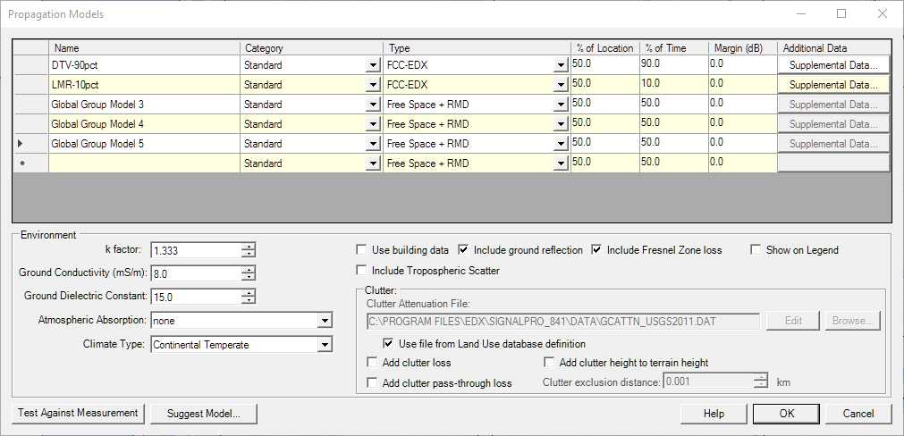
- First, set up two FCC propagation models, one for 90% of time (DTV) and the other for 10% of time (LMR), similar to below. Select any one of the FCC model Types appropriate for your study requirements. The two models can be given any Name you choose:
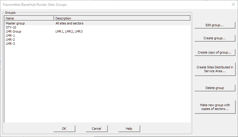
2. Next, add/position the desired transmitters on the map and then create a transmitter group for the DTV site as well as for other LMR transmitters. This can be done either individually for each LMR site or specific LMR sites can be placed in their own group as needed. Example below:
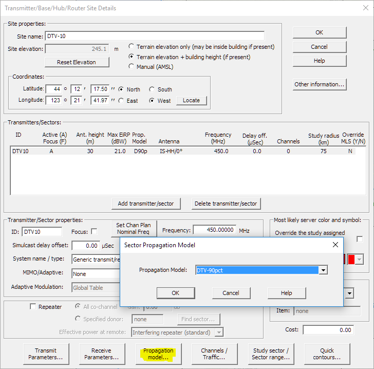
3. Edit each transmitter site (or use the spreadsheet editor to submit a bulk change), select the Propagation Model button and in the dialog box, assign the desired Propagation Model (either DTV-90pct or LMR-10pct) to each transmitter. If you choose, you can also change the Transmitter ID, to make it more descriptive and match the Site Name (DTV-10). Do this for both the DTV and LMR sites. Example for transmitter DTV-10:
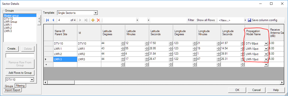
Example for changing transmitter Propagation Model Name using the EDX Spreadsheet editor (RF Systems>Spreadsheet Editors>Sectors Data):
4. Create an area study for the DTV transmitter and also for the LMR Group using "Field strength at remote" Study Name and select the appropriate transmitter group for the Primary Transmitter group. Example for DTV-10:
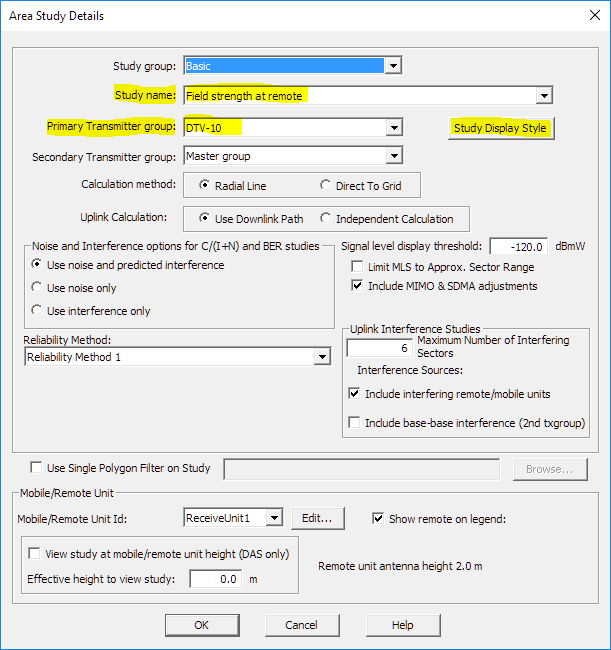
5. Click the Study Display Style button in the Area Study Details Dialog box which opens the Area Study Style dialog box. From the Study display type drop-down list, select "FCC-type contours". Example:
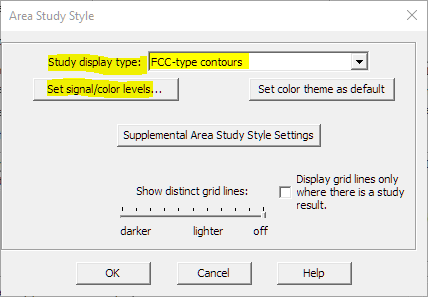
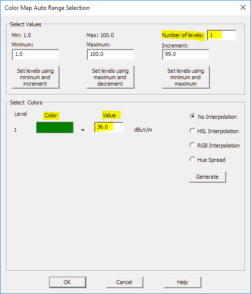
6. Click the Set signal/color levels button in the dialog box and in the Color Map Auto Range Selection dialog box, change the Number of levels value to 1 (for one contour), then click on the Color area to change the color (if desired) and lastly, change the level Value to match the contour field dBµV/m for that transmitter or transmitter group, in this case 36 dBuV/m for DTV-10:
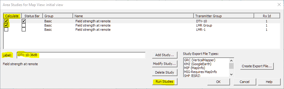
7. Finally, click OK to exit all the dialog boxes until you return to the Area Studies for Map View: initial view dialog box. In the Label field, provide an appropriate name for the recently created “Field strength at remote" area study. Continue to add studies for the remaining transmitters/groups and assigning labels, level colors and level values. Example below shows the label for the DTV-10 area study:
When all studies have been created and labeled, click OK to exit this dialog box and save the changes.
Creating the contours for the DTV and LMR sites
Now, let's say we want to see if there is any contour interference between DTV-10 and the LMR group (composed of LMR-1, LMR-2 and LMR-3).
- open the Areas Studies for Map View dialog box, check the Calculate button for just those two studies and then click the Run Studies button (see screen capture above). Once the studies complete, the map view will display the contours for each transmitter group. Example below:
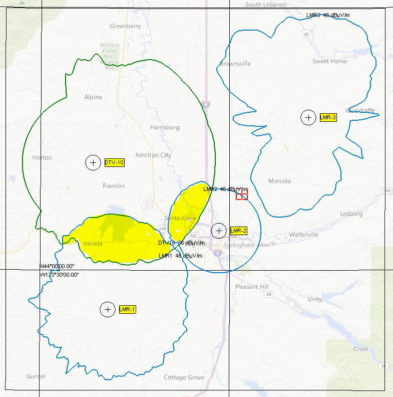
2. The Map Layer now shows the Area study contour results for the DTV-10-36dB and LMR_Group-46dB studies. The areas, which have been highlighted in yellow, show where there is contour overlap for the DTV-10 site and two of the LMR sites (LMR-1 and LMR-2).
Contour files
In the area study, if you select the FCC contours, the program no longer uses the area study code that other propagation models use. Instead, it uses the code from the Interference Contours Study, and creates a ".ctr" file directly. This was never designed to have multiple independent contour “maps/studies.” Each FCC contours study overwrites the previous one, so an FCC contours area study can only have one current ".ctr" file.
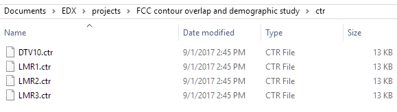
The contour files, which are created when running an area study, reside in the project folder in the \ctr\ subfolder.
Example of a portion of the contents of the DTV10.ctr file. Note the Number of contours (1) and the Contour Levels dBµV/m of 36:
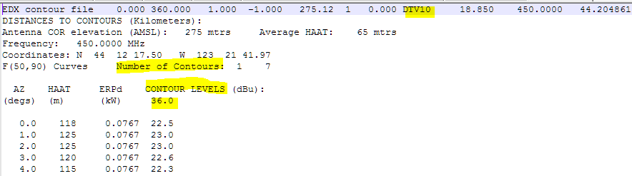
Each of the contour files from your studies will have a similar format/set up.
Set up and configuration to run the Demographic study for the contour overlap
Demographic data base
Ensure the Demographic data base is configured for your project (Databases>Demographic), otherwise you will not be able to run the demographic study. Once the database is configured, it can be displayed on the map layer by adding a "demographic data" layer (Add Layer) in the Map Layers dialog box. With the "demographic data" layer highlighted, by clicking the Style button, the Demographic attribute to plot can be selected from the drop-down list. In this example select "Housing units". Also, for the Type of demographic plot select "flat grid" from the drop-down menu. Click OK to save and exit. The transparency of the "demographic data" layer can be adjusted as desired in the Map Layers dialog box.
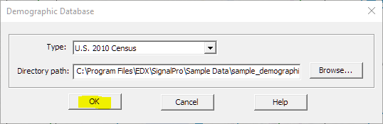
- If not configured, open the Demographic Database dialog box and click the Browse button to navigate to your demographic file folder.
- Select the folder containing the demographic database files and click the OK button.
- In the Type drop-down list, select the appropriate census year and then click the OK button to save your selections and exit the dialog box.
Example below:
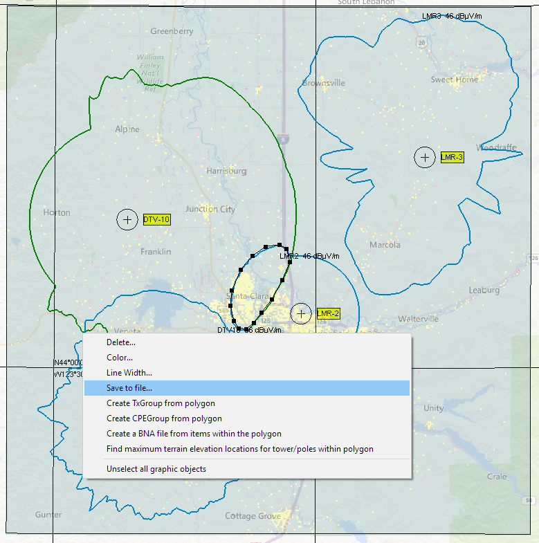
4. On the map layer showing the area study results, use the polygon tool (Draw>Polygon) to draw around the areas of overlap to create a polygon bna file.
5. Right click on the polygon line to open a contextual menu and select “Save to file” and save the file in the \ctr\ folder of your project using a ".bna" extension (The file was saved as dtv10-lmr2-overlap.bna). Depending on the complexity of the overlap area, you may need to create more than one polygon bna file. The example below shows a polygon for the overlap between DTV-10 and LMR-2 (with demographic information represented in yellow on the map layer):
6. Repeat the above steps for any other overlap contours on which you want to run demographic studies
Running the Demographic Study
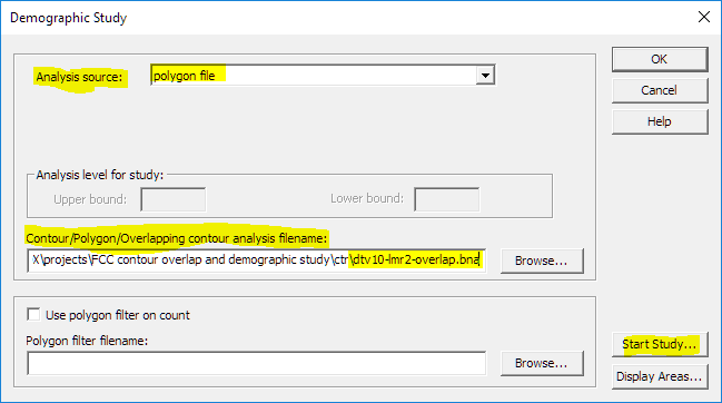
In the Demographic Study dialog box (Studies>Demographic Studies), select "polygon file" from the drop-down list as the Analysis source and then in the Contour/Polygon/Overlapping contour analysis filename field, browse to one of the polygon bna files you created (in this example,dtv10-lmr2-overlap.bna), open it and click the Start Study button.
2. The Demographic Study Results dialog box will display.
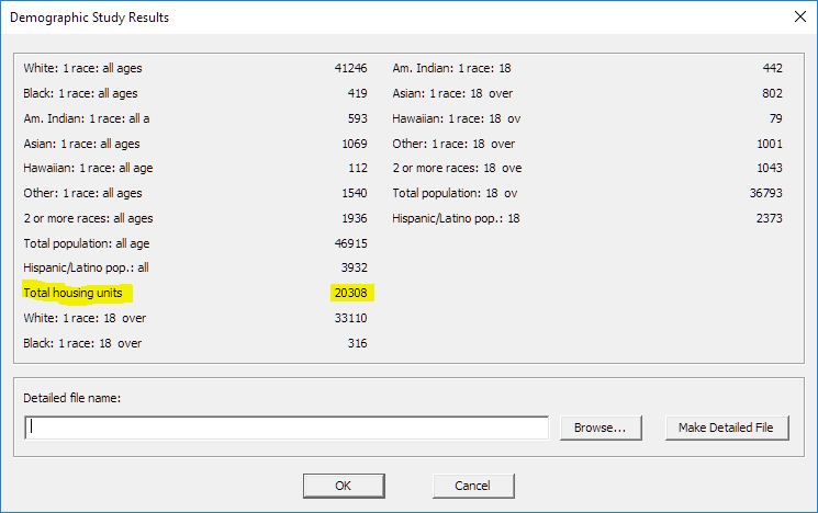
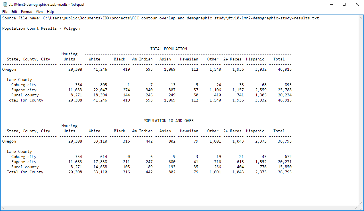
3. To save the results as a file, enter a name for the file, click the Make Detailed File button (see results output below) or note the value of the field in which you are interested (example: Total housing units).
4. Click OK to close the dialog box and return to the Demographic Study dialog box. Repeat the above for any other polygon bna files. Now you have the total demographic information for all the LMR overlaps in the DTV contour area.
Related articles